
Bifacial photovoltaic (PV) modules have moved from a premium niche to the default choice for utility-scale solar. Most large fixed-tilt and single-axis tracker projects entering construction today specify bifacial glass-glass modules, and the technology now accounts for the majority of new utility-scale capacity in major markets.
The appeal is simple to state and surprisingly hard to deliver: a bifacial module captures sunlight on both faces, so a single rack of modules can produce meaningfully more energy from the same footprint. The trouble starts when a developer treats the manufacturer’s headline “bifacial gain” as a fixed bonus to bake into the energy model. It is not. The rear-side contribution is a function of the site, the mounting geometry, and the quality of the build – and getting it wrong on either the optimistic or conservative side has real consequences for yield, electrical design, and bankability.
This article is for the engineers, developers, and EPC contractors who size, model, and build these systems. We’ll work through how bifacial modules actually generate the extra energy, what controls the gain, how the rear-side current changes electrical design, and how to model the system credibly enough to satisfy a lender.
What Bifacial PV Systems Are
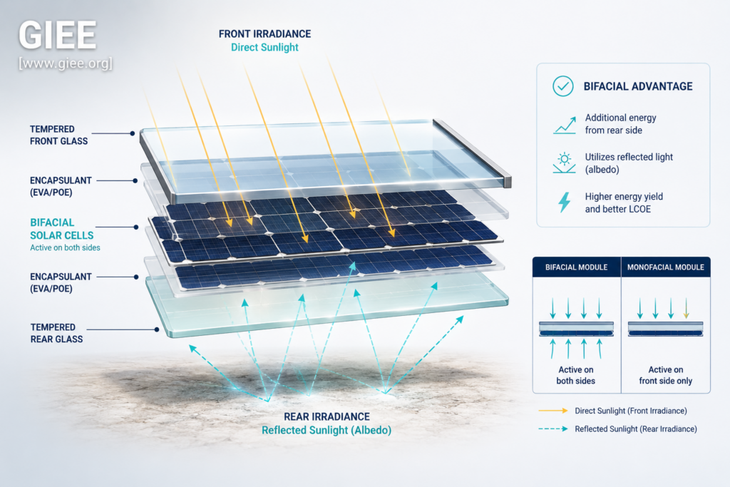
A monofacial module has an opaque backsheet. Light that reaches the rear is absorbed or wasted. A bifacial module replaces that backsheet with glass or a transparent polymer and uses cells that are photovoltaically active on both surfaces, so light striking the rear is also converted to power.
Modern cell architectures make this practical. PERC (passivated emitter and rear contact), TOPCon (tunnel oxide passivated contact), and heterojunction (HJT) cells all expose a rear junction that responds to incident light, differing mainly in how much of the rear light they use.
That “how much” is captured by the bifaciality factor – the ratio of the cell’s rear-side efficiency to its front-side efficiency, measured under identical irradiance.
Typical values by cell type:
- PERC: φ ≈ 0.70–0.75
- TOPCon: φ ≈ 0.80–0.85
- HJT: φ ≈ 0.90–0.95
A higher bifaciality factor means more of the rear-side light becomes usable power. It does not, by itself, tell you how much energy the system will gain – that depends on how much light reaches the rear in the first place.
How Bifacial Modules Work
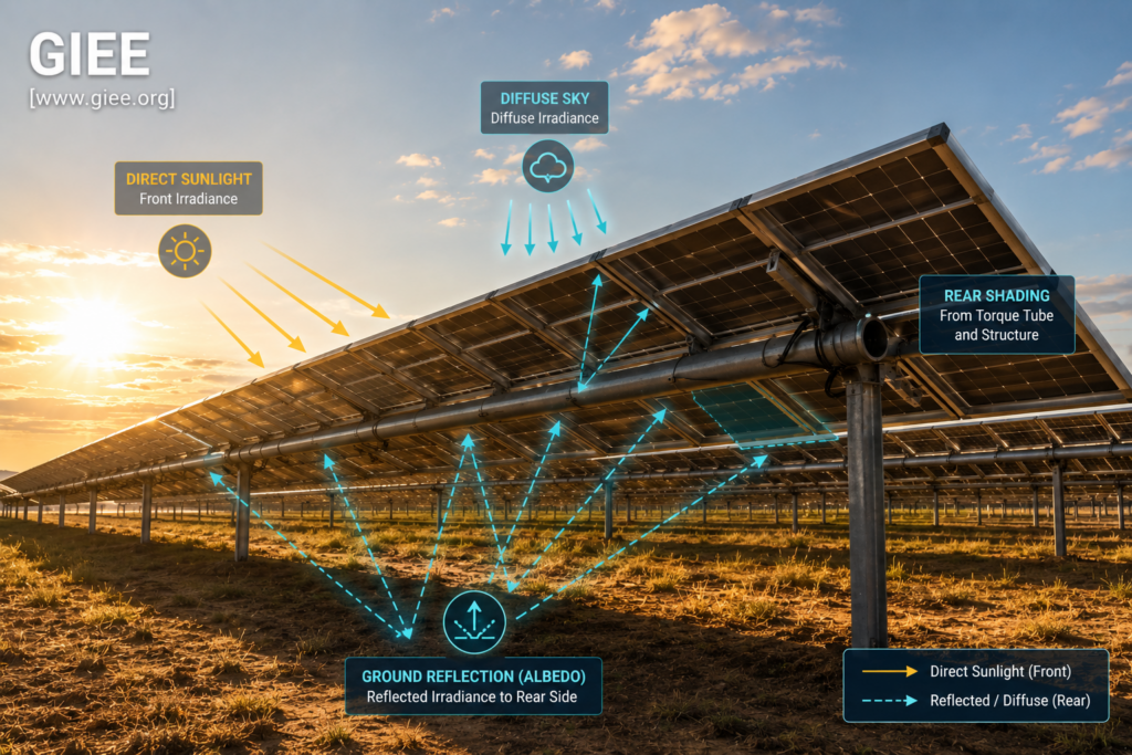
The front face behaves exactly like a conventional module: it sees direct beam plus diffuse sky irradiance in the plane of the array (POA). The difference is the rear, which sees a much weaker and far less uniform irradiance field.
A useful way to think about the module’s electrical behavior is the effective irradiance – the front-side POA irradiance plus the rear-side irradiance, weighted by the bifaciality factor:
The rear-side term is where almost all the engineering judgment lives. Front irradiance is predictable from well-validated irradiance models. Rear irradiance is non-uniform, view-factor dependent, and sensitive to everything happening underneath and around the array.
Sources of Rear-Side Irradiance
Rear irradiance comes from three contributions, in rough order of importance for a typical ground-mount system:
- Ground-reflected irradiance (albedo). The dominant source. Sunlight hitting the ground in front of and beneath the array reflects upward onto the rear face. This is what makes albedo the single biggest lever on bifacial gain.
- Diffuse sky irradiance. Part of the rear face has a view of the sky (especially near module edges and at the top of the array), contributing scattered light independent of ground reflection.
- Reflections from surroundings. Adjacent structures, equipment, or even neighboring module rows can reflect or, more often, block rear light.
Against these gains sit the losses: the racking, torque tube, purlins, junction boxes, and cabling all cast shadows on the rear face, and the ground directly under the array receives less direct sun than the open ground between rows.
Bifacial Gain and What Controls It
Bifacial gain is the additional annual energy a bifacial system produces relative to an otherwise identical monofacial system.
In practice, bifacial gain for well-designed utility-scale systems typically falls in the 5–15% range, occasionally higher over very reflective ground such as desert sand or snow. The wide range is the whole point: the same module can deliver 6% on one project and 12% on another. Several factors drive that spread.
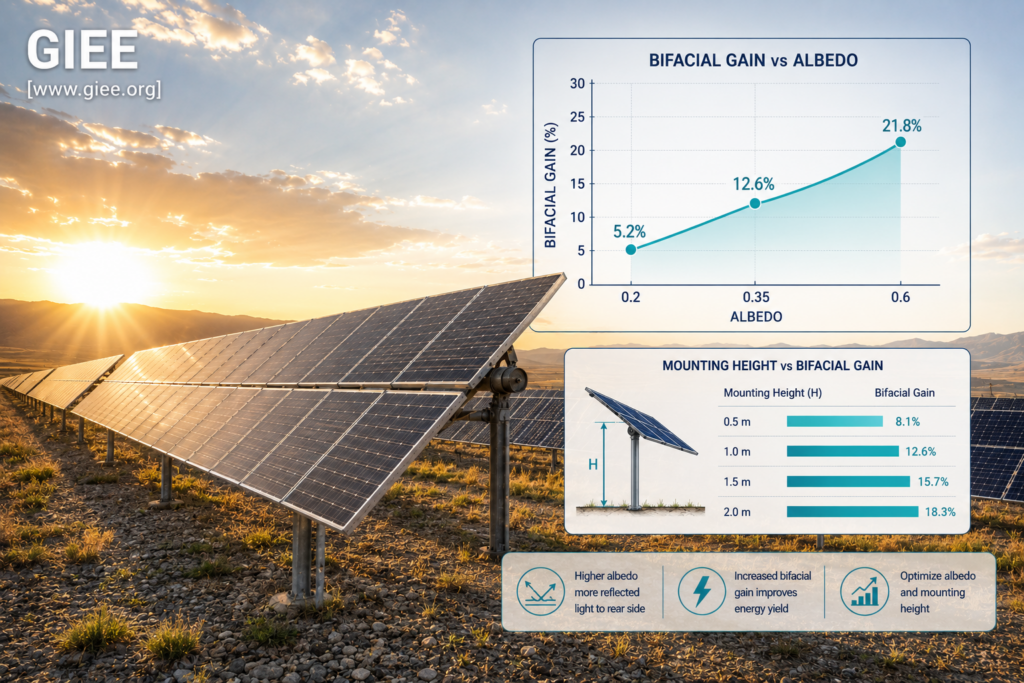
Albedo
Albedo – the fraction of incident light a surface reflects – is the strongest single driver of bifacial gain.
Representative values:
- Green grass / vegetation: 0.15–0.25
- Dry bare soil: 0.17–0.23
- Concrete: 0.25–0.35
- Desert sand: 0.30–0.40
- White gravel / membrane: 0.50–0.70
- Fresh snow: 0.60–0.90
Practical example – albedo effect. Consider the same fixed-tilt bifacial array modeled over three ground covers. Over grass (ρ ≈ 0.20), the rear contribution might add roughly 6% to annual yield. Move that array onto desert sand (ρ ≈ 0.35) and the gain can climb toward 10–11%. A reflective white membrane on a commercial rooftop (ρ ≈ 0.60) can push the gain higher still. Nothing about the module changed – only the ground beneath it.
Mounting Height
Raising the array increases the rear face’s view of reflective ground and reduces the influence of the shadowed strip directly beneath the modules. The result is more – and more uniform – rear irradiance.
Practical example – mounting height. Raising the bottom edge of a fixed-tilt array from roughly 0.5 m to 1.5 m of ground clearance can lift bifacial gain by several percentage points, often from the mid-single digits toward double digits, with diminishing returns above about 1.5–2 m. The trade-off is structural: taller posts and stronger wind-load design add cost, so the optimum is an economic decision, not just a yield-maximizing one.
Row Spacing and Ground Coverage Ratio
Ground coverage ratio (GCR) is the array area divided by the land area. Lower GCR – wider row spacing – exposes more ground to direct sun between rows, increasing the reflected light available to the rear face.
Wider spacing improves bifacial gain but uses more land and more cabling, and reduces energy density per acre. This is one of the clearest examples of why bifacial design is a system-level optimization rather than a module choice.
Rear-Side Shading and Installation Quality
Every object behind the module costs energy. A wide torque tube on a tracker, closely spaced purlins, surface-mounted junction boxes, and untidy DC cabling all shade the rear cells. Because rear irradiance is already a fraction of front irradiance, these losses bite harder in relative terms.
Design Considerations and Engineering Challenges
Designing a bifacial system well means optimizing the whole geometry, not just selecting a high-bifaciality module:
- Tracker vs. fixed-tilt. Single-axis trackers generally amplify bifacial gain because they keep the front face well-illuminated through the day and continually expose fresh ground to direct sun. Most large bifacial projects pair the two.
- Tracker structure. A slim, offset torque tube preserves more rear irradiance than a wide central tube directly behind the cells.
- Ground preparation. Where economics allow, light-colored gravel or engineered ground cover raises albedo. For commercial rooftops, a reflective membrane can be a low-cost gain.
- Edge and end effects. Modules at row ends and array edges see more rear light, producing non-uniform output across the array that the model should capture.
- Soiling on two faces. Rear glass soils differently than front glass and is harder to clean; account for it in the O&M plan.
The honest summary: bifacial introduces more design variables, and each one couples to the others. That complexity is the cost of the extra energy.
Electrical Sizing Implications
The point engineers most often underestimate is that bifacial modules don’t just produce more energy over the year – they produce more current during operation. The rear-side contribution raises short-circuit current (Isc) and maximum-power current (Imp) above the front-only nameplate values.
This affects several design decisions:
- Conductor and combiner sizing. String and DC collection conductors must carry the elevated current. Sizing strictly off the monofacial nameplate rating can leave conductors and combiner boxes under-rated.
- Overcurrent protection. Fuse and disconnect ratings should reflect the bifacial-boosted current, consistent with the relevant electrical code (in the US, NEC Article 690 current calculations).
- Inverter loading and clipping. The added DC production interacts with the DC-to-AC ratio (inverter loading ratio, ILR). A bifacial array can clip more often at the inverter than a monofacial array of the same nameplate, which both affects energy harvest and must be modeled.
Practical example – current sizing. Suppose a string is built from modules with a front-side Isc of 13.5 A. Under high-albedo conditions the rear contribution can raise the operating short-circuit current by on the order of 5–10%, pushing effective Isc toward 14.2–14.9 A. Conductors, fuses, and combiner inputs sized on the bare 13.5 A figure now sit closer to their limits than the designer intended. The fix is straightforward – apply a bifacial current factor early in the DC design – but only if it isn’t overlooked.
Performance Modeling and Bankability
Because the rear-side contribution is geometry- and site-dependent, modeling it credibly is central to financing a project.
Industry tools handle bifacial at different levels of fidelity. PVsyst implements a view-factor (2D) bifacial model that most developers use for energy estimates, while ray-tracing approaches – such as NREL’s open-source bifacial_radiance – capture row-to-row and edge effects in more detail for studies that justify the extra effort. Whatever the tool, the rear-side estimate carries more uncertainty than the front-side estimate, and lenders know it.
The annual energy yield itself follows the familiar form, with the bifacial contribution folded into the effective irradiance:
Practical example – yield improvement scenario. Take a 100 MW utility-scale plant whose monofacial design models 200 GWh/yr. A credibly modeled 9% bifacial gain raises that to roughly 218 GWh/yr – about 18 GWh of additional annual energy from the same land and interconnection. Over a 30-year life, that difference is large enough to move the project’s economics materially, which is exactly why the gain assumption gets scrutinized so closely.
That scrutiny ultimately lands on the levelized cost of energy.
Bifacial modules carry a modest cost premium over monofacial and may require taller structures, but they add energy to the denominator without proportionally increasing the numerator. In most utility-scale settings the result is a lower LCOE – provided the modeled gain holds up in operation.
Best Practices for Maximizing Bifacial Performance
For practitioners optimizing real projects, the highest-leverage actions are consistent across sites:
- Raise and characterize albedo. Measure it on site, and improve it with gravel or reflective ground cover where the economics justify it.
- Optimize mounting height and GCR together. Treat them as coupled variables in a yield-versus-cost optimization, not independent rules of thumb.
- Minimize rear obstructions. Specify slim torque tubes, rear-friendly junction box placement, and disciplined cable management.
- Size electrical BOS to bifacial current. Apply the bifacial current factor to conductors, fuses, combiners, and inverter loading from the start.
- Model conservatively and validate. Use a view-factor or ray-tracing model, apply realistic uncertainty bands, and reconcile modeled gain against measured production once operating.
Future Outlook
Bifacial is no longer the differentiator – it’s the baseline. As TOPCon and HJT cells displace older architectures, average bifaciality factors are climbing toward 0.85 and beyond, raising the ceiling on achievable rear-side gain. The pairing of bifacial modules with single-axis trackers is now standard practice for utility-scale solar, and elevated and agrivoltaic designs are opening new ways to manage albedo and ground use deliberately rather than accepting whatever the site offers.
The remaining frontier is modeling confidence. As ray-tracing tools, validated field data, and standardized bifacial test methods mature, the uncertainty band around rear-side energy will tighten – and with it, the conservatism lenders apply. The technology question is largely settled. The engineering question that still separates good projects from mediocre ones is whether the design actually captures the gain the module makes possible.
That is the right way to think about bifacial PV: not as a fixed bonus stamped on a datasheet, but as energy you earn through site selection, geometry, electrical discipline, and honest modeling. The module gives you the opportunity. The engineering decides how much of it you keep.
Designing or modeling a bifacial project and want to go deeper on hosting capacity, interconnection current limits, or performance modeling? Explore GIEE’s related guides and courses on utility-scale PV engineering.