Key Takeaways
- All three problems share one root cause: real conductors have resistance and reactance, so moving current through them costs both energy and voltage.
- Conductor losses scale with the square of current (P = I²R). This single fact explains why we transmit at high voltage and why poor power factor is so expensive.
- Voltage drop along a line depends on both resistance and reactance, and it limits how far and how heavily any feeder can be loaded.
- A power factor below unity forces extra current for the same real work, compounding both losses and voltage drop.
- Power factor correction and disciplined loading are among the cheapest efficiency and reliability gains available to a working engineer.
Electrification is pushing more current through infrastructure that was sized decades ago. Data centers, EV charging depots, heat pumps, and new industrial loads are loading feeders and transformers closer to their limits, while distributed energy resources (DER) change where and how power flows. In that environment, three classic problems that an engineer might think of as solved are resurfacing with real consequences: power losses, voltage drop, and power factor.
This article explains those three problems from first principles. It is written for working electrical engineers who want a clean mental model they can apply on the job, and for early-career engineers who want to go deeper than the one-line definitions in a textbook. By the end, you should be able to explain why each problem occurs, estimate its magnitude, and connect it to a real decision – conductor sizing, capacitor placement, or how hard you can load a feeder.
One Root Cause, Three Symptoms
Start with the uncomfortable truth that every practical conductor is imperfect. A real line, cable, or winding has an impedance, usually written as Z = R + jX, where R is the resistance and X is the reactance. Resistance comes from the physical material opposing the flow of electrons. Reactance comes from the magnetic and electric fields the current sets up as it flows. Neither is a defect to be engineered away; both are unavoidable properties of carrying alternating current through metal in the real world.
Once you accept that conductors have impedance, the three problems follow directly. Resistance turns part of the delivered energy into heat: that is power loss. Impedance, acting against the current, produces a difference between the voltage you send and the voltage that arrives: that is voltage drop. And when the load draws current that is out of phase with the voltage, part of that current does no useful work but still has to be carried: that is the power factor problem. The three are not separate phenomena. They are three views of the same physics, and in a real system they feed one another.
1. Power Losses: Why Current Costs Energy
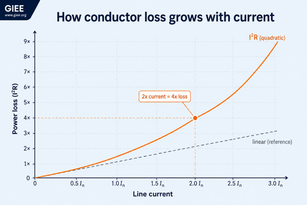
When current flows through resistance, electrical energy is converted into heat. This is Joule heating, and it is the dominant loss mechanism in any current-carrying conductor. The power dissipated does not scale with current; it scales with the square of current.
The squared term is the whole story. Double the current and the loss quadruples. Halve the current and the loss falls to a quarter. This is why the entire transmission system is built around high voltage. For a given amount of real power, P = √3 × V × I × cosφ in a three-phase system, so raising the voltage lets you carry the same power with proportionally less current. Less current, squared, means dramatically less loss. A 765 kV line moving the same megawatts as a 138 kV line carries roughly one-sixth the current and suffers a small fraction of the heating loss.
It helps to separate the two families of loss in real equipment. Copper losses (the I²R term) rise and fall with load, since they depend on current. Core losses in transformers and motors – hysteresis and eddy currents in the iron – are driven by the applied voltage and frequency and stay roughly constant whenever the equipment is energized, even at no load. A lightly loaded distribution transformer can spend most of its life dominated by core loss; a heavily loaded feeder cable is dominated by copper loss. Knowing which regime you are in tells you where to spend money.
Combined transmission and distribution losses in the United States run about 5% of all electricity delivered each year [EIA]. At national scale that is more than 200 TWh of generation lost as heat in the wires – energy that was produced, paid for, and never reached a load.
In an industrial plant, copper loss shows up as warm cable trays, oversized conductor bills, and energy charges that do not match production. Long runs to remote loads (a pump house, a crusher, a far end of a yard) are the usual culprits, because resistance is proportional to length. The practical lever is almost always the same: reduce the current the conductor has to carry, or shorten and fatten the conductor. The chart below shows why current reduction is the more powerful lever.
2. Voltage Drop: Why the Far End Sags
The same impedance that wastes energy also robs voltage. As current flows along a line, the voltage at the receiving end is lower than the voltage at the source. The magnitude of that drop depends on the current, the line impedance, and crucially on the phase relationship between voltage and current. A useful working approximation for the drop along a three-phase line is given below.
Equation 2 carries a practical lesson that catches people out: whether resistance or reactance dominates the drop depends on the voltage level. On a distribution feeder, conductor resistance is often comparable to or larger than reactance, so the R cosφ term leads and real power flow drives most of the drop. On a transmission line, reactance is much larger than resistance, so the X sinφ term leads and reactive power flow drives the drop. That is why distribution engineers obsess over conductor size and feeder length, while transmission engineers manage voltage with reactive devices such as capacitor banks, reactors, and static VAR compensators.
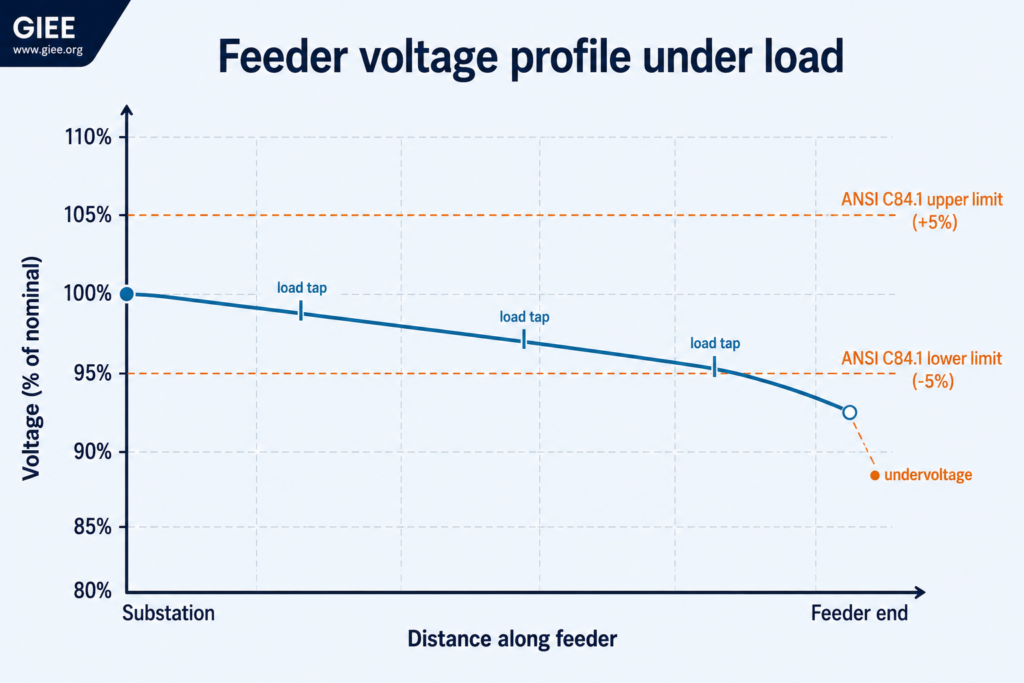
Voltage drop is not just an efficiency nuisance; it is a reliability and equipment problem. Induction motor torque falls with the square of the terminal voltage, so a motor at the sagging end of a loaded feeder may struggle to start a high-inertia load or may stall and trip. Lighting dims, electronic power supplies work harder and run hotter, and process controllers can misbehave on a marginal supply. The standard that bounds all of this in North America is ANSI C84.1.
Picture a long rural distribution feeder. At the substation the voltage sits near nominal, but each load tapped along the way draws current, and every meter of conductor adds impedance. By the time you reach the last customer at the end of a heavily loaded feeder, the voltage may have sagged below the lower ANSI limit, especially during peak demand. Utilities manage this with voltage regulators, load tap changers, and reactive support, but the underlying driver is always Equation 2. The voltage profile below shows the shape of the problem.
3. Power Factor: Current That Does No Work
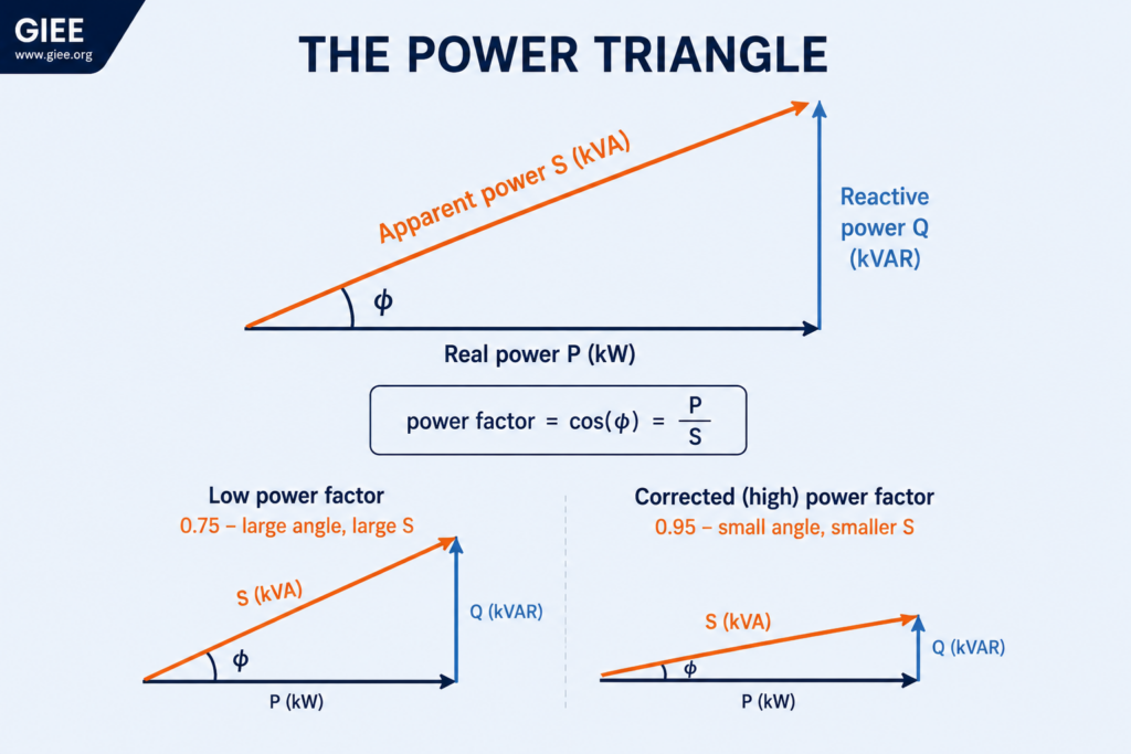
The third problem is the most misunderstood, because it involves a kind of current that delivers no net energy yet still loads every component in its path. Inductive equipment – induction motors, transformers, welders, older fluorescent ballasts – needs current to build and collapse magnetic fields each cycle. That current, called reactive power (Q, measured in kVAR), flows back and forth without doing useful work. The real, useful power is P (kW), and the total the system actually has to carry is the apparent power S (kVA).
These three quantities form a right triangle: S² = P² + Q². Power factor is simply the ratio of useful power to total power, cosφ = P / S, where φ is the angle between current and voltage. A purely resistive load has a power factor of 1.0 and draws only the current it needs. An inductive load has a power factor below 1.0, and the lower it goes, the larger the apparent power and the larger the current for the same real work.
Here is where the three problems join hands. The current a load draws is set by Equation 3, and power factor sits in the denominator.
A typical industrial plant full of partially loaded induction motors might run at a power factor around 0.75. The plant still does its real work, but it pulls far more current than the work requires, and the utility, which has to size transformers and lines for apparent power, often bills a demand or power factor penalty as a result. Installing capacitor banks supplies the reactive power locally, near the motors, so the system upstream no longer has to carry it. The worked example shows what correcting from 0.75 to 0.95 actually buys.
How the Three Problems Compound
In a real system these problems rarely appear alone, and the worst conditions stack them. Consider the far end of a long, heavily loaded distribution feeder serving an industrial customer at poor power factor. The low power factor inflates the current (Equation 3). The inflated current raises the I²R heating along the whole feeder (Equation 1) and deepens the voltage drop to the customer (Equation 2). The depressed voltage then makes the customer’s motors draw still more current to deliver the same torque, which feeds the cycle again. Each problem amplifies the others.
The encouraging flip side is that the levers are shared too. Reducing current at the source – through power factor correction, load balancing, or shifting demand off the peak – attacks all three at once. Keeping conductors short and adequately sized limits both loss and drop. Holding voltage near nominal keeps motor currents low. An engineer who internalizes that current is the common villain, and that loss grows with its square, has most of the intuition needed to diagnose a tired feeder or an underperforming plant.
Conclusion
Power losses, voltage drop, and power factor are not three unrelated topics from three different textbook chapters. They are three consequences of one fact: real conductors have impedance, and current flowing through impedance costs energy and voltage. Once you see I²R, the voltage-drop relation, and the power triangle as different angles on the same physics, the practical priorities fall into place – keep current down, keep conductors short and sized right, correct your power factor, and hold voltage near nominal. As electrification pushes more current through aging infrastructure, the engineers who treat these fundamentals as live design constraints, not settled history, will build the systems that stay efficient and reliable under load. To go deeper on the distribution side, see GIEE’s guide to hosting capacity analysis and our material on conductor sizing and voltage-drop budgeting.