
Introduction
Almost every consequential decision in a PV system how many modules go in a string, which inverter clears the project, whether a commissioned array is actually delivering nameplate, and why a string is underperforming three years in traces back to a single relationship: the module’s current as a function of its voltage. The I–V curve is not a teaching aid. It is the contract between the silicon and the rest of the system, and the engineer who reads it fluently catches in minutes what a SCADA energy report buries for a season.
The trouble is that the datasheet I–V curve is a single point in a large space. It is measured at Standard Test Conditions (STC: 1000 W/m², 25 °C cell, AM1.5 spectrum) conditions a module almost never sees in the field. Real arrays operate across a continuum of irradiance and temperature, with mismatch, soiling, partial shading, and slow degradation reshaping the curve. This guide treats the I–V curve as a working instrument: how to read its shape, how it moves with environment, and how to translate that movement into string limits, inverter windows, commissioning acceptance criteria, and fault signatures.
Key Takeaways
- Voc at minimum cell temperature, not STC, sets your maximum string length. Crystalline-silicon Voc rises roughly 0.3 %/°C as temperature drops; cold-morning open-circuit voltage is the number that must clear the inverter and system voltage limit per NEC 690.7.
- Vmp at maximum cell temperature sets your minimum string length. If hot-day Vmp falls below the inverter’s MPPT lower bound, the array operates off its maximum power point and sheds energy you already paid for.
- The slopes of the curve are diagnostic. Shallow slope near Voc points to rising series resistance (connectors, solder, terminations); a tilted, non-flat segment near Isc points to a shunt path (PID, cell defect, ground fault).
- A field trace means nothing until it is translated to STC. Per IEC 60891, compare measured curves to expected curves only after correcting for the irradiance and temperature at the moment of measurement otherwise you will chase phantom faults.
- Partial shading produces multiple maxima, not just a lower peak. Bypass-diode conduction creates a stepped I–V curve and a multi-peak P–V curve; only global MPPT finds the true optimum.
- In a series string, the lowest-current module governs. Mismatch losses are a current-limiting phenomenon the curve of the weakest module is felt by the whole string.
What the I–V Curve Actually Represents
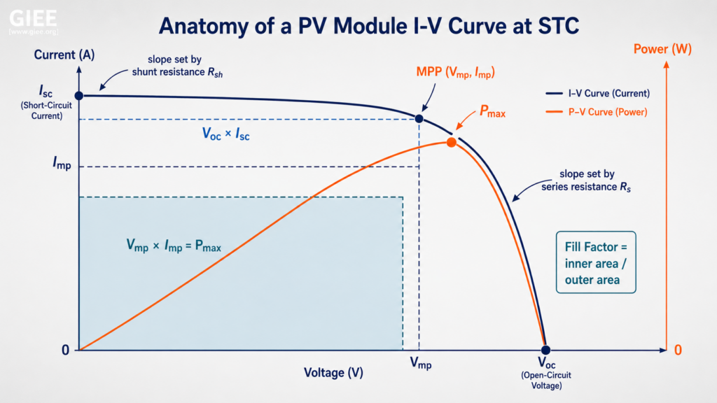
Five points define the working envelope, and the engineering value lies in how they move and what they imply not in their dictionary definitions.
Definitions
Short-circuit current (Isc) is the current at zero terminal voltage. It is set almost entirely by photogenerated current and therefore tracks irradiance nearly linearly. Isc is the cleanest proxy for “how much light is reaching the cells right now,” which is exactly why a depressed Isc in a field trace points first to soiling, shading, or an irradiance-reference error rather than to a module defect.
Open-circuit voltage (Voc) is the voltage at zero current. It depends only logarithmically on irradiance but strongly and negatively on temperature. Voc is the parameter that dictates electrical safety and equipment survival, because the worst case a cold, sunny, open-circuit morning is when it peaks.
Maximum power point (Vmp, Imp) is the single operating point where the product V·I is largest. Vmp typically sits near 0.80–0.82·Voc and Imp near 0.90–0.95·Isc for a healthy crystalline module, but those ratios drift with temperature and degradation, which is the whole reason MPPT windows need design margin.
Maximum power (Pmax = Vmp·Imp) and the fill factor tie the curve’s geometry to its quality:
Fill factor measures how “square” the knee is. A healthy c-Si module runs FF ≈ 0.74–0.82. A falling fill factor with Voc and Isc largely intact is the field signature of resistive losses creeping in, and it is invisible to a metric that only watches energy yield.
When a string underperforms, separate the symptom before you theorize. Down Isc → light is the problem (soiling/shading). Down Voc → count your cells (substring/diode/temperature). Square knee gone soft → resistance. Curve tilted up near Isc → shunting. The four signatures rarely lie.
The Physics Behind the Curve Shape
A PV cell is a large-area photodiode, and its terminal behavior is captured well by the single-diode model:
where IL is the light-generated current, I0 the diode saturation current, n the ideality factor, Vt = kT/q the thermal voltage (≈ 25.9 mV per junction at 300 K), Rs the lumped series resistance, and Rsh the shunt resistance. Each term governs a region of the curve, and that is what makes the model useful in the field rather than merely in a simulator.
Near short circuit, the diode term is negligible and the curve is dominated by IL and the shunt path. A finite Rsh tilts the otherwise-flat segment upward current bleeds off as voltage rises. Near open circuit, the exponential diode term takes over and the curve plunges; here Rs sets the slope, because the voltage drop I·Rs steepens the rolloff and rounds the knee. In an ideal cell (Rs → 0, Rsh → ∞) the curve would be perfectly rectangular with FF → 1. Every real loss mechanism pushes FF down by attacking one of these two regions, which is precisely why slope reading is a diagnostic act.
Irradiance scales the whole curve almost vertically: IL is directly proportional to incident irradiance, so Isc rides up and down with the sun. Voc moves only logarithmically, because it is governed by the ratio IL/I0 inside the exponential doubling irradiance adds only a few hundred millivolts across a typical 60- or 72-cell module.
Maximum Power Point in Real Systems
The datasheet curve shows one MPP. The field shows a moving target. As irradiance and temperature shift through the day, Vmp and Imp wander across the I–V plane, and the inverter’s job is to keep the array pinned to that wandering point.
Maximum power tracking exploits a simple condition: at the MPP, dP/dV = 0. Perturb-and-observe (P&O) and incremental-conductance (IncCond) algorithms walk the operating voltage up and down, watching whether power rises or falls, and settle at the knee. The consequence for design is that the inverter does not operate the array at Voc or Isc it commands a voltage somewhere on the knee and holds it. The array’s actual operating point is therefore wherever the MPPT controller places it, and that point must remain inside the inverter’s MPPT voltage window for the tracker to do its job.
This is where theory meets a hard constraint. The MPPT window is a finite band for example, roughly 200–800 V on a typical three-phase string inverter, capped by an absolute maximum input voltage of 1000 V or 1500 V. If Vmp climbs above the window on a frigid morning, the inverter rides at the window edge and loses MPP. If Vmp sinks below the window on a hot afternoon, the inverter undervolts, tracking collapses, and production clips. Designing the string is therefore the act of keeping Vmp inside that band across the full temperature range the site will see not at STC.
Effects of Irradiance and Temperature
These two variables move the curve in nearly orthogonal directions, and conflating them is the root of most string-sizing errors.
Irradiance acts on current. To good approximation:
so the curve stretches and compresses vertically with the sun. Voc shifts only modestly adding roughly (n·Ns·kT/q)·ln(G/1000) for an Ns-cell module which is why a heavily shaded or dawn condition shows collapsed current but still-substantial voltage. For energy yield this is intuitive: power scales nearly with irradiance. For design it means irradiance rarely threatens voltage limits.
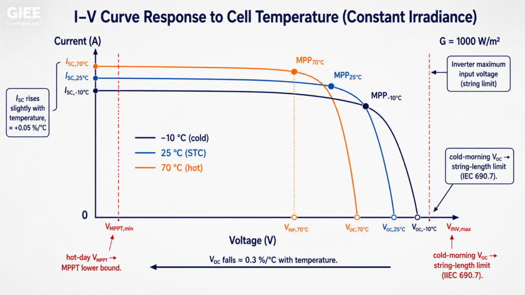
Temperature acts primarily on voltage, and it is the dominant design driver. For crystalline silicon, the temperature coefficients run approximately:
- Voltage: β ≈ −0.27 to −0.35 %/°C (Voc falls as the cell heats)
- Current: α ≈ +0.04 to +0.06 %/°C (Isc rises slightly)
- Power: γ ≈ −0.35 to −0.45 %/°C
The current rise is trivial; the voltage fall is decisive. Corrected Voc is:
Take a module with Voc,STC = 49.5 V and β = −0.29 %/°C at a site whose extreme minimum is −10 °C. The correction factor is 1 + (−0.0029)(−35) = 1.10 a 10 % rise to ≈ 54.5 V per module. That single number governs how many modules clear the system limit:
NEC 690.7 requires maximum PV system voltage to be calculated using the lowest expected ambient temperature for the site (commonly the ASHRAE extreme-minimum or 2 % value), applied via the module’s temperature coefficient or the 690.7(A) correction table. Designing on STC Voc is both non-compliant and unsafe.
At the hot end, the same physics squeezes Vmp downward. A 1.5 °C/W mounting on a 40 °C ambient day can push cell temperature past 65–70 °C, dropping Vmp by 12–18 % from its STC value. That hot-day Vmp is the number that must stay above the MPPT minimum the lower bookend of string sizing.
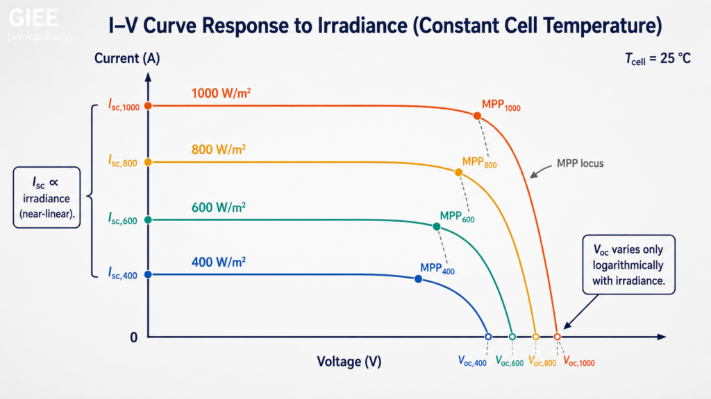
Figure 2. With cell temperature held constant, irradiance scales the curve almost vertically: Isc varies nearly linearly with irradiance while Voc shifts only logarithmically, so the maximum power point moves mainly downward as irradiance falls.
Non-Ideal Behavior in the Field
The clean single-knee curve survives only as long as every cell sees the same conditions. Real arrays violate that assumption constantly.
Partial shading and bypass diodes. When a cell is shaded, it produces less current than its series neighbors, which try to push their full current through it. The shaded cell goes into reverse bias and would dissipate destructively without protection. The substring bypass diode conducts to carry the current around the shaded group, and in doing so it carves a step into the I–V curve. Each conducting bypass diode adds a step; the corresponding P–V curve develops multiple local maxima. A conventional MPPT can lock onto a local peak and leave real power on the table which is why global MPPT (periodic full-window sweeps) exists. The lesson for design: shading is not a linear derate, and a module-level model that ignores diode topology will mispredict it.
Mismatch losses. In a series string every module carries the same current, so the lowest-current module sets the string’s operating current a current-limiting bottleneck. In parallel, the lowest-voltage element pulls the others down. Mismatch arises from manufacturing tolerance, uneven soiling, differential degradation, and orientation differences on complex roofs. Tight current binning, string-level grouping by performance, and where mismatch is structural module-level power electronics (DC optimizers or microinverters) are the standard mitigations.
Multiple MPPs and string-level effects. Because steps and mismatch combine, a long string under non-uniform conditions can present a genuinely multimodal P–V surface. At the array level this interacts with the inverter’s tracking strategy and DC/AC ratio: an oversized DC array clips at the top of the curve under high irradiance, which is an intentional design trade, not a fault but it must be distinguished from the involuntary clipping caused by an out-of-window Vmp.
Reading a stepped or soft-kneed field curve as “low irradiance.” Low irradiance scales the curve down cleanly; it does not put steps in it or round the knee. Steps mean shading or diode activity; a rounded knee with intact Voc/Isc means series resistance. Translate to STC first, then interpret the shape.
Engineering Use Cases
The I–V curve is the common currency across four routine engineering tasks.
String sizing. This is the canonical two-sided constraint. The upper bound comes from cold Voc: N_max·Voc(T_min) must clear the inverter’s absolute maximum input and the system voltage rating per NEC 690.7. The lower bound comes from hot Vmp: N_min·Vmp(T_max) must stay above the inverter’s MPPT minimum so tracking holds on the hottest expected operating day. A defensible string length lives between these two numbers with margin on both ends and both numbers come straight off temperature-corrected curve points, never STC.
Inverter selection. The curve dictates the match. The inverter’s MPPT window must envelop the array’s Vmp excursion from coldest-operating to hottest-operating conditions; its maximum input voltage must survive cold-morning Voc; its maximum input current per MPPT input must accommodate Imp plus bifacial gain and any high-irradiance enhancement. The DC/AC ratio is then a deliberate choice about how much of the high-irradiance top of the curve to clip in exchange for better low-light utilization.
Performance validation. At commissioning, a field I–V trace per IEC 62446-1 is compared to the expected curve from the module model and the measured plane-of-array irradiance and cell temperature. Acceptance is judged on translated parameters Isc, Voc, Pmax, and fill factor within tolerance after correction. This baseline is what every future trace is measured against, so capturing it correctly at commissioning is non-negotiable.
Fault diagnostics. Once a baseline exists, the shape tells the story. The diagnostic map is consistent and worth committing to memory:
| Curve symptom | Most likely cause |
|---|---|
| Isc down, shape intact | Soiling, shading, irradiance-reference error |
| Voc down, Isc intact | Open substring, failed bypass diode, fewer active cells |
| Knee rounded, FF down | Rising series resistance: connectors, solder, terminations |
| Near-Isc segment tilts up | Shunt path: PID, cell defect, ground fault, low Rsh |
| Steps / notches in curve | Partial shading or bypass-diode conduction |
Common Engineering Mistakes
These recur across commissioning reports and field investigations, and each one traces back to misreading or misapplying the curve.
Sizing strings on STC Voc. The most expensive error in the book. Using 25 °C Voc instead of cold-corrected Voc undercounts the worst-case voltage by ~10 %, producing strings that overvolt the inverter on the first cold sunny morning nuisance trips at best, equipment damage and an NEC 690.7 violation at worst.
Ignoring hot-day Vmp. The mirror error. A string sized only against the upper voltage limit can collapse below the MPPT minimum at 65–70 °C cell temperature, so the array silently underproduces every hot afternoon while passing a casual STC sanity check.
Comparing field traces without translation. Holding a measured curve up against the STC datasheet curve, with no correction for the irradiance and cell temperature at the moment of measurement, manufactures faults that do not exist. IEC 60891 translation is not optional rigor; it is the difference between a real anomaly and an artifact of the weather.
Misreading a series-resistance signature as low irradiance. A rounded knee with healthy Isc and Voc is resistive loss, not a cloud. Treating it as irradiance hides degrading terminations until they fail sometimes thermally.
Trusting nameplate fill factor indefinitely. Fill factor drifts down with age as Rs creeps up and Rsh creeps down. A performance model that assumes constant FF will overstate yield as the array matures and will mask the slow onset of resistive or shunt degradation.
Modeling shading as a linear derate. Because bypass diodes create steps and multiple maxima, a uniform percentage derate misestimates both energy loss and the inverter’s ability to find the global peak. Shading needs topology-aware modeling, not a flat haircut.
Mismatching the irradiance reference plane. A reference cell or pyranometer not coplanar with the modules or of a different spectral and angular response corrupts the translation and, with it, every parameter judged against it. The sensor must represent what the array sees.
The Bottom Line
The I–V curve is the most information-dense object in a PV system, and it earns its keep at both ends of a project’s life. At design time, two temperature-corrected points off that curve cold Voc and hot Vmp bound the string length and force the inverter match; everything else in the DC design is negotiation inside those limits. In operation, the curve’s shape is a fault dictionary: current tells you about light, voltage tells you about cells, the knee tells you about resistance, and the near-short-circuit slope tells you about shunting. The engineer who insists on translating every field trace to STC before interpreting it, and who sizes strings against environmental extremes rather than nameplate conditions, will design systems that clear inspection, hold their MPP across the year, and surface degradation while it is still a connector and not yet an outage.