Key Takeaways
- Voltage drop is the loss of potential along a conductor caused by its resistance and, in AC, its reactance – it is set by current, conductor properties, and length, not by the source voltage.
- The working formulas differ by system: DC uses ΔV = I·R; single-phase and three-phase AC add the reactive term (R·cosφ + X·sinφ).
- The practical targets most engineers design to are 3% on a branch circuit and 5% total (feeder plus branch) – echoed by NEC informational notes and IEC 60364-5-52.
- Long runs, low voltages, high currents, and poor power factor are the four conditions that push drop out of spec; the fix is almost always a larger conductor or a higher distribution voltage.
- On long DC runs such as solar strings, even a fraction of a percent compounds into real lost energy over a 25-year plant life – so PV designers target tighter limits than the code minimum.
Introduction
Ask any commissioning engineer about the failures that show up late on a project, and voltage drop will be near the top of the list. The cable was the right ampacity. The breaker coordinated. The single-line looked clean in review. Yet the motor at the far end of a 150-metre feeder refuses to start cleanly, or the lighting contractor reports that a long branch circuit measures several volts low under load. Nothing has “broken.” The conductors are simply doing what conductors do – converting a slice of the delivered voltage into heat along the way.
Voltage drop sits at the intersection of physics and economics. The physics is unavoidable: push current through a real conductor and you lose voltage in proportion to its impedance. The economics is where the engineering lives. You can almost always solve a drop problem by throwing copper at it, but copper is expensive, heavy, and harder to terminate. The discipline is in delivering acceptable voltage at the load while spending the least on conductor, conduit, and labour – and doing it within the limits a code official will accept.
This guide is written for the practising electrical engineer who already knows Ohm’s law and wants the working knowledge that sits one layer above it: the correct formulas for DC, single-phase, and three-phase systems; how reactance and power factor change the answer; the code limits that govern the sign-off; and three fully worked examples – a residential run, an industrial motor feeder, and a solar PV DC cable – that mirror the calculations you actually perform on the job.
What Voltage Drop Is
Voltage drop is the difference between the voltage available at the source and the voltage that actually arrives at the load, measured under operating current. It is not a fault, a leak, or a sign of bad workmanship. It is the predictable consequence of current flowing through the finite impedance of every conductor, joint, and termination between the supply and the equipment.
The mechanism is straightforward. A copper or aluminium conductor has resistance proportional to its length and inversely proportional to its cross-sectional area. When load current flows, that resistance develops a voltage across the conductor exactly as it would across any resistor. The energy represented by that voltage does not vanish – it leaves the system as heat in the cable, which is precisely why oversized currents in undersized conductors are both a voltage-drop problem and a thermal one.
Two consequences fall straight out of this relationship and explain most of what engineers see in the field. First, drop grows linearly with run length – double the distance and you double the drop. Second, drop falls as conductor area rises, which is the lever designers reach for first. Resistivity itself is not constant, either: copper’s resistance climbs by roughly 0.4% per degree Celsius, so a conductor running hot at full load carries meaningfully more resistance than the 20 °C table value suggests.
Why Voltage Drop Matters in Real Systems
Excessive voltage drop is rarely catastrophic on its own, which is part of what makes it dangerous – it degrades performance quietly until something downstream misbehaves. The effects are specific to the load type, and a good designer thinks about the load before reaching for a formula.
Motors are the classic victim. Torque in an induction machine scales with the square of the terminal voltage, so a 10% drop during a hard start can cut available starting torque by nearly 20%. A motor that cannot develop enough torque draws locked-rotor current for longer, heats up, and may trip on overload or fail to accelerate its load at all. The running case is gentler but not harmless: a chronically under-volted motor draws higher current to deliver the same shaft power, runs hotter, and ages faster. It is worth being precise about timing: the large drop seen during a start is temporary – it lasts only the few seconds the machine spends accelerating – but it is critical, because that brief window is exactly when the motor needs full voltage to develop starting torque.
Electronic and resistive loads have their own sensitivities. Switch-mode power supplies compensate by drawing more current as voltage sags, which simply moves the problem upstream. Incandescent and halogen lighting dims visibly and shifts colour temperature. Heating elements lose output as the square of voltage. Across a facility, the same drop that is invisible at one outlet becomes a measurable energy penalty when summed over hundreds of circuits running for thousands of hours.
In practice, the most common real-world driver is distance. A solar array on the far corner of a site, a pump house at the end of a long agricultural feeder, a crane at the end of a gantry busway – these are where engineers quickly run into the limits, because length is the one term in the equation that the site geography, not the designer, controls.
A sustained 5% voltage drop on a feeder serving resistive heating load translates into roughly a 10% loss in delivered heat output – because resistive power scales with the square of voltage. The drop you tolerate is rarely the loss you actually pay.
The Fundamental Equations
Three forms cover almost everything an engineer needs day to day. They share the same logic – current times impedance – but differ in how they account for the return path and for AC reactance. Get the system type right before you pick the formula; using a single-phase equation on a three-phase feeder is one of the most common spreadsheet errors in the trade.
Direct current
DC is the simplest case. There is no reactance to consider, so only resistance matters. The voltage lost in one conductor is current times that conductor’s resistance.
One point trips up newcomers. EQ 1 gives the drop across a single conductor, but a real DC circuit is a complete loop – current flows out along the supply conductor and returns along the second – so the load feels the drop of both. The voltage drop of the complete DC loop is therefore ΔV = 2 · I · R, where R is the one-way resistance of one conductor. Keep the two quantities distinct: I · R is the single-conductor drop, while 2 · I · R is the full circuit (loop) drop the load actually experiences – and the loop value is the one you compare against a limit. This same factor of two reappears in the single-phase AC case, for exactly the same reason.
Single-phase AC
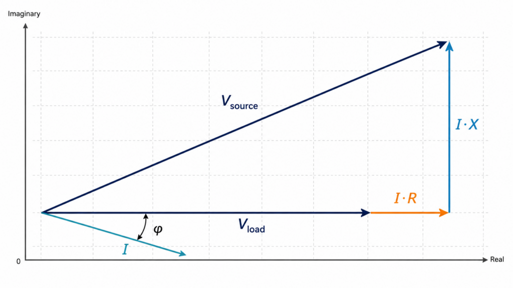
In AC systems, the conductor’s inductive reactance joins resistance to form impedance. The voltage drop now depends on the load’s power factor, because the resistive and reactive components of the drop combine according to the phase angle between voltage and current. The standard approximate formula – accurate enough for the great majority of low-voltage work – is:
The leading 2 again accounts for both the line and the neutral conductor, so EQ 2 – like the DC loop expression – already gives the complete-circuit drop, not a single-conductor value. Notice what happens at unity power factor: sinφ becomes zero, the reactance term disappears, and the expression collapses back to the familiar resistive drop. The reactance term only earns its keep when power factor is poor or conductors are large – which is exactly the industrial-feeder situation. For those larger conductors, take R and X from AC impedance tables (for example, NEC Chapter 9, Table 9) rather than from pure DC resistance, because skin effect and conductor proximity raise the effective AC resistance above the DC value.
Three-phase AC
A balanced three-phase system has no current in the neutral, so the factor of two is replaced by √3, which relates the line-to-line voltage to the per-phase drop. Otherwise the structure is identical.
Finally, the number that matters for code compliance is rarely the volts themselves but the drop expressed as a fraction of nominal voltage. Percentage voltage drop normalises the result so it can be compared against a limit regardless of system voltage.
AC vs DC Voltage Drop
The practical difference between the two comes down to one word: reactance. In DC, current is steady and there is no changing magnetic field around the conductor, so inductance plays no role – resistance alone sets the drop. This is why DC voltage-drop work is conceptually clean but unforgiving: with no reactance to hide behind, the only levers are conductor size, length, and operating current.
AC introduces inductive reactance because the alternating current sets up an alternating magnetic field that opposes changes in current. For small conductors at low voltage, reactance is small relative to resistance and is often neglected. For large conductors, long parallel runs, and higher voltages, reactance can equal or exceed resistance, and ignoring it produces optimistic – and wrong – answers. The spacing and arrangement of conductors also matters, since reactance depends on the geometric mean distance between phases. This is also the regime where the AC resistance itself exceeds the DC value, so pull both R and X from AC cable tables rather than from a DC resistance figure.
Power factor is the other AC-only consideration. The same current at the same conductor produces a larger drop at lagging power factor than at unity, because the reactive component of the drop adds in. A motor load at 0.85 lagging will show a noticeably higher feeder drop than a resistive load of identical current – a fact that surprises engineers who size cables from current alone. This is also why power-factor correction near a load reduces both line current and the reactive contribution to drop, improving voltage at the load on two fronts at once.
Factors Affecting Voltage Drop
Strip the formulas down and five variables drive the outcome. Understanding which ones you can move – and at what cost – is most of the design judgement.
Conductor length. The dominant factor on most projects, and usually fixed by site layout. Because drop is linear in length, halving a run by relocating a panel often beats upsizing the cable, and it is worth raising during layout review rather than after the routing is set.
Cross-sectional area. The primary design lever. Doubling area roughly halves resistance and therefore halves the resistive drop. The cost is non-linear – larger cable, larger conduit, harder terminations, and more weight on cable tray – so the engineering is in stepping up only as far as the limit requires.
Current magnitude. Drop scales directly with load current. This is why motor starting (six to eight times running current) and inrush events define the worst-case drop, even when the steady-state figure looks comfortable.
Conductor material. Aluminium has about 1.6 times the resistivity of copper for the same area, so an aluminium conductor must be sized up by roughly two standard sizes to match copper’s drop. It remains attractive on long runs and large feeders because, per unit of conductance, it is cheaper and far lighter – a genuine cost-versus-performance trade-off rather than a simple “copper is better” choice.
Power factor and reactance. As covered above, lagging power factor and larger conductor reactance raise AC drop. Temperature also belongs here, and it is worth being exact about which temperature: what counts is the conductor’s actual operating temperature, not the ambient air alone. A loaded conductor heats itself through its own I²R losses, so it runs well above room temperature – and because copper’s resistance climbs about 0.4% per °C, the same circuit drops more at its 75–90 °C operating temperature than the 20 °C table value implies.
| Factor | Effect on drop | Designer’s lever? |
|---|---|---|
| Run length | Linear increase | Limited – set by layout |
| Conductor area | Inverse – bigger area, less drop | Primary lever |
| Load current | Linear increase | Sometimes (staging, soft start) |
| Material (Cu vs Al) | Al ≈ 1.6× the resistance of Cu | Yes – cost/weight trade-off |
| Power factor | Worse PF, higher AC drop | Yes – PF correction |
| Temperature | ~0.4%/°C rise in Cu resistance (operating temp, not ambient) | Indirect – ampacity, derating |
Practical Design Examples
The formulas earn their place only when you run real numbers through them. The three examples below use round but realistic figures and a copper resistivity of 0.0175 Ω·mm²/m. They follow the sequence you would use at the desk: establish the current, find the conductor resistance, apply the right equation, then judge the result against a limit.
Voltage Drop Limits – Codes and Standards
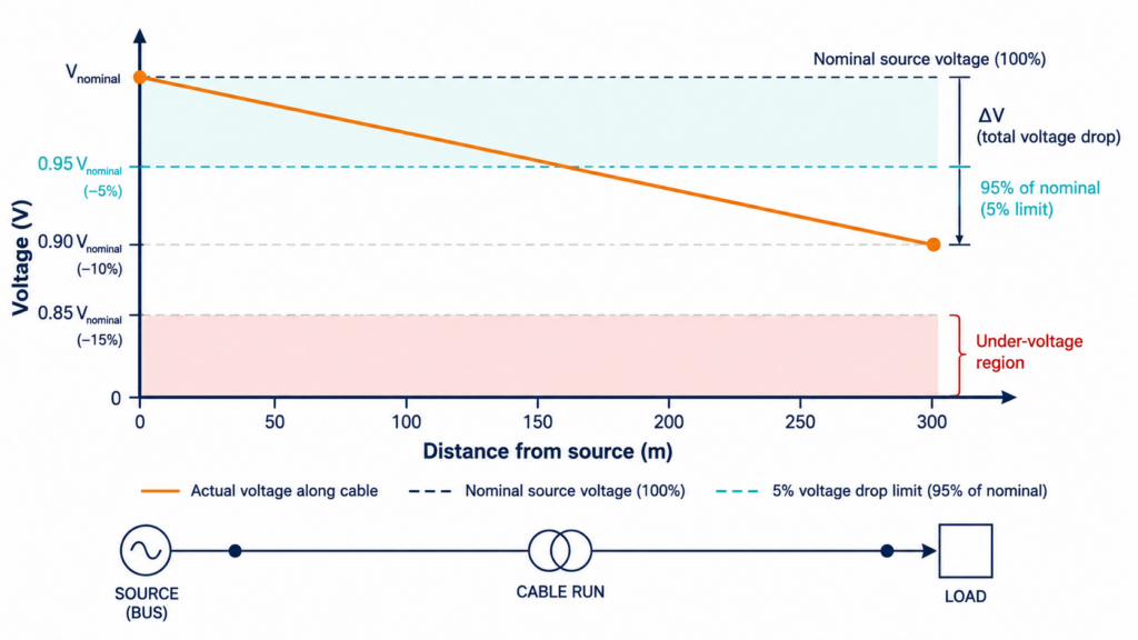
Two number pairs govern most low-voltage design, and they are worth committing to memory: 3% on a branch circuit and 5% total from the service to the load. The nuance is that these are recommendations in some codes and hard requirements in others, so the engineer has to know which framework applies in the jurisdiction.
In the United States, the National Electrical Code does not impose a mandatory voltage-drop limit for general wiring. Instead, Informational Notes to NEC 210.19(A) (branch circuits) and 215.2(A) (feeders) recommend sizing conductors so that branch-circuit drop does not exceed 3%, and the combined feeder-plus-branch drop does not exceed 5%, to provide “reasonable efficiency of operation.” Because these are informational notes, they are not directly enforceable – but they are the de facto industry standard, they appear in most specifications, and certain applications (notably sensitive electronic equipment and some fire-pump and emergency circuits) carry stricter, enforceable limits elsewhere in the code.
Internationally, IEC 60364-5-52 takes a similar position. Its informative Annex G recommends that voltage drop between the origin of an installation and any point of utilisation not exceed 3% for lighting and 5% for other uses when the installation is supplied directly from a public low-voltage network. Higher allowances apply for installations fed from a private transformer, recognising that the designer controls more of the supply chain in that case.
Mitigation Strategies
When a calculation comes back over limit, engineers have a small, well-understood toolkit. The art is choosing the cheapest effective option for the specific situation.
Increase conductor size. The default move, and often the right one for short overruns. Stepping up one or two standard sizes restores margin without changing the system architecture. The penalty is material cost, conduit fill, and termination effort, all of which climb steeply at large sizes.
Raise the distribution voltage. The most powerful lever for long runs, because at higher voltage the same power moves at lower current, and drop scales with current. Distributing at 480 V instead of 240 V, or running a PV plant at 1500 V DC instead of 600 V, can cut percentage drop dramatically. This is why utilities push voltage up for transmission and why long site feeders are routinely run at the highest practical voltage and transformed down near the load.
Shorten the run. Relocating a panel, sub-panel, or combiner closer to the load attacks the length term directly and often costs nothing but coordination during layout. It is the most overlooked option because it must be caught early, before routing is fixed.
Correct power factor. On AC systems with lagging loads, adding capacitors near the load reduces line current and the reactive contribution to drop simultaneously. For large motor installations this can be more economical than upsizing a long feeder.
Use a different material or parallel conductors. Switching from aluminium to copper, or running multiple conductors in parallel per phase, increases effective area. Parallel runs are common on large feeders where a single conductor would be unwieldy to pull and terminate.
Impact on System Performance and Efficiency
It is tempting to treat the code limit as the goal and stop there, but voltage drop is also an efficiency story, and the two views can diverge. Every volt dropped across a conductor is power dissipated as heat – power the customer paid for and the load never received. That loss equals current squared times resistance, so it grows faster than the drop itself and is heavily weighted toward the most heavily loaded circuits.
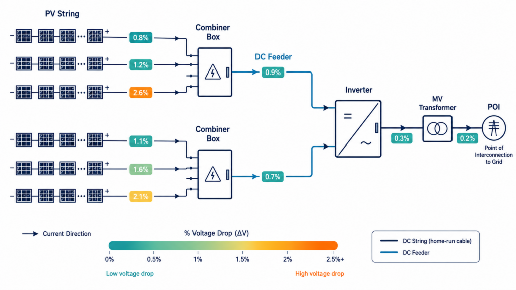
For circuits that run continuously, the economic case for tighter design strengthens. A feeder sitting at the 5% limit during peak hours is dissipating real money in conductor heating year-round. On a solar plant, the calculus is starker still: DC-side losses recur every sunlight hour for the life of the array, so a fraction of a percent of extra drop, multiplied across a 25-year horizon, can justify a noticeably larger conductor on net-present-value grounds alone. This is why PV and other generation projects routinely design to drop limits well below what any safety code requires – the driver is yield, not compliance.
There is also a stability dimension on larger systems. Voltage drop is one contributor to the overall voltage profile a network operator must hold within tolerance. On distribution feeders with high distributed-generation penetration, the interaction between load-driven drop and generation-driven voltage rise becomes a hosting-capacity question – a reminder that the same physics scales from a single branch circuit up to the feeder and beyond.
Best Practices
The habits that separate clean designs from the ones that come back at commissioning are not complicated; they are mostly about checking the right cases at the right time.
Calculate drop at the design stage, not after the cable schedule is locked. Size for ampacity first, then verify drop, and be ready to upsize – the two checks are independent and the larger of the two governs. For motor and other high-inrush loads, always run the starting case explicitly, because the steady-state figure will mislead you. Use AC resistance and reactance values at operating temperature for anything above small conductor sizes, rather than 20 °C DC values, so the analysis reflects the cable as it actually runs at full load. Keep a clear record of which voltage reference you used and apply the percentage limit consistently against it. And on generation and continuously loaded circuits, evaluate drop against lifetime energy cost, not only the code minimum – the cheapest cable on day one is frequently the expensive choice over twenty years.
Conclusion – An Engineering Perspective
Voltage drop rewards engineers who respect it early and quietly punishes those who treat it as an afterthought. The physics is fixed – current through real impedance loses voltage, every time – but the response is entirely a design choice. Knowing the three working equations, understanding why reactance and power factor reshape the AC answer, and checking the worst case rather than the average one will resolve the great majority of situations you meet in practice.
The deeper skill is holding two questions in mind at once: will this pass the code limit? and is this the right amount of copper to buy? Those questions usually point the same direction, but on long runs, continuous loads, and generation projects they diverge, and that is where good judgement earns its keep. Treat the 3% and 5% figures as a floor, run the numbers for the case that actually stresses the circuit, and design with margin for the temperature your cable will really see. Do that, and voltage drop stops being the problem that surfaces at commissioning and becomes one more variable you closed out at the desk.
If you want to take the distribution-side analysis further – hosting capacity, DER-driven voltage rise, and the planning studies where these calculations scale up to the feeder – explore GIEE’s coursework on distribution system analysis and DER integration.